
Useful tip: To make sure that all the scenario data is valid, click the Check button in the General data section.

Your company shows steady revenue growth but still struggles to improve profitability? In many cases, the issue isn’t the sales volume. The bottleneck may lie in the hidden logistics costs that come from serving certain customers or delivering specific products.
This is where applying cost to serve analysis to logistics can be an eye-opener for many businesses, giving insights for a more comprehensive optimization plan and unlocking even greater profitability. By allocating logistics, warehousing, transportation, and service costs directly to customers and products, companies can uncover hidden losses. And the good news is that it became possible to do in anyLogistix after the 3.4.2 release and a new dedicated Cost to serve experiment.
In this blog post, we’ll explore how to use this new experiment and identify profitability issues across the supply chain. We’ll also walk through a practical example to demonstrate how to set up, run, and interpret a cost to serve analysis in practice.
Contents:
Our example features Apex Auto Parts GmbH, a regional automotive components distributor based in Munich, Germany. The company supplies five product types, including components such as spark plugs and oil filters, to 24 independent repair shops and major customers across Germany.
Despite stable revenue growth, the company’s net profit has slowed significantly in recent months. Reports indicate that serving certain clients consumes a disproportionate share of operational resources and logistical costs. But the company lacks sufficient visibility to determine the exact sources and drivers of these inefficiencies. And that’s why they turned to anyLogistix to find proof for their assumptions.
The current supply chain configuration includes a detailed 4-week demand plan with variable weekly order patterns, which should be added to the Demand table in the software. The supply chain has the following structure, which we replicate using the input tables in anyLogistix.
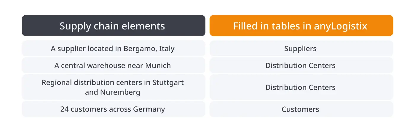
Different input tables in anyLogistix (click to enlarge)
Overall, in this example, 16 input tables are used to represent all the necessary details of the operations and ensure the accuracy of experiments. Once the scenario data is prepared, the project is ready for optimization.
Useful tip: To make sure that all the scenario data is valid, click the Check button in the General data section.
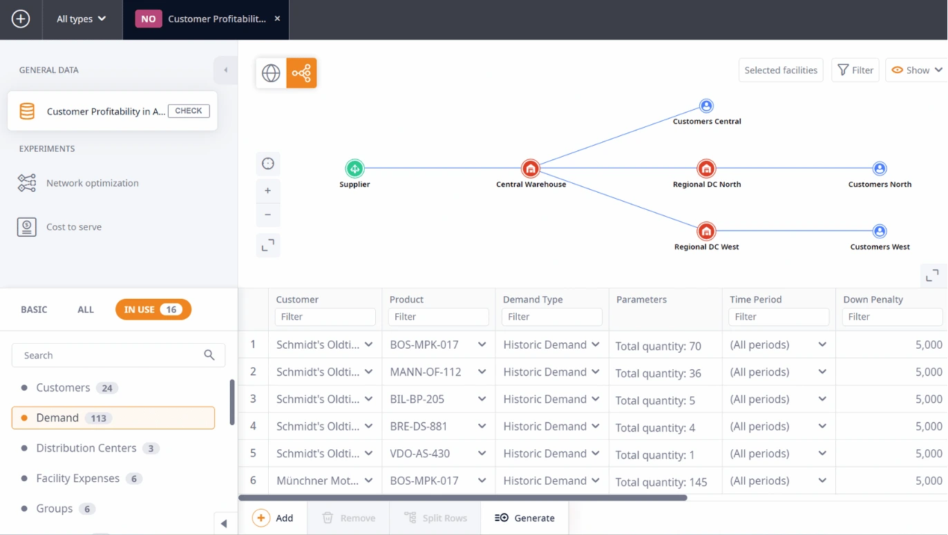
Supply chain configuration and in-use input tables in anyLogistix (click to enlarge)
Before performing cost to serve analysis, we first need to evaluate the baseline supply chain performance. To do this, let’s run one iteration of a standard Network optimization experiment for the current scenario configuration.
The experiment calculates key operational KPIs such as:
We can explore the current state of the supply chain in the results output table and in the configurable KPI panel. These initial results indicate that the company’s operations are profitable overall, with a net profit margin of 9.5%.
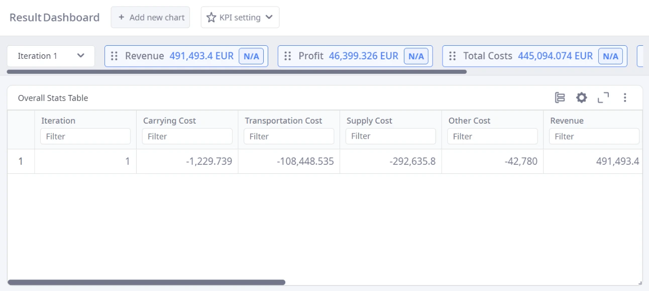
Result dashboard and the KPI panel in anyLogistix (click to enlarge)
While this represents a stable level of profitability, it can be insufficient for long-term business growth. More importantly, these aggregated numbers do not reveal which customers or products are driving losses.
This is where the Cost to serve experiment becomes critical. Running a cost to serve analysis in anyLogistix allows users to identify hidden operational costs and evaluate optimization opportunities that are not visible in standard network optimization results.
As we now have the baseline results of the Network optimization experiment, let’s run the Cost to serve analysis on top of it, using the same scenario data. To do this, simply click on the experiment icon and choose the following in the settings:
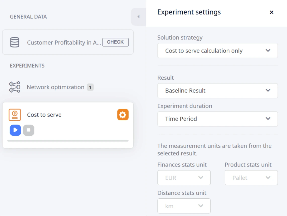
Experiment setting of the Cost to serve analysis (click to enlarge)
After running the experiment, anyLogistix provides several analytical ways that help uncover hidden profitability patterns and support cost to serve optimization decisions.
The Cost to serve light table contains aggregated operational and financial indicators for every customer-product combination. By sorting the table by ascending Profit, total values, it becomes immediately clear that several deliveries generate negative profit.
In our case, most of the losses are associated with the BRE-DS-881 product.
This way, we quickly isolate a problematic product and identify where operational costs exceed generated revenue.
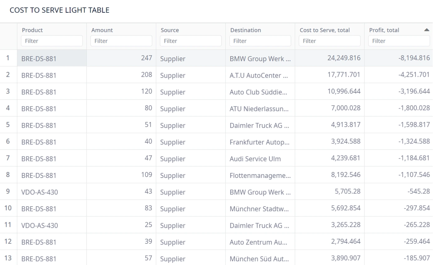
Cost to serve light results table (click to enlarge)
Now let’s have a look at the Cost to serve by product table that aggregates the same data, but at the product level. The analysis reveals that the BRE-DS-881 product indeed generates substantial losses for the company. The gap between Revenue per item and Cost to serve per item approaches €20.
This level of visibility helps distinguish between isolated customer issues and broader product-level profitability problems.
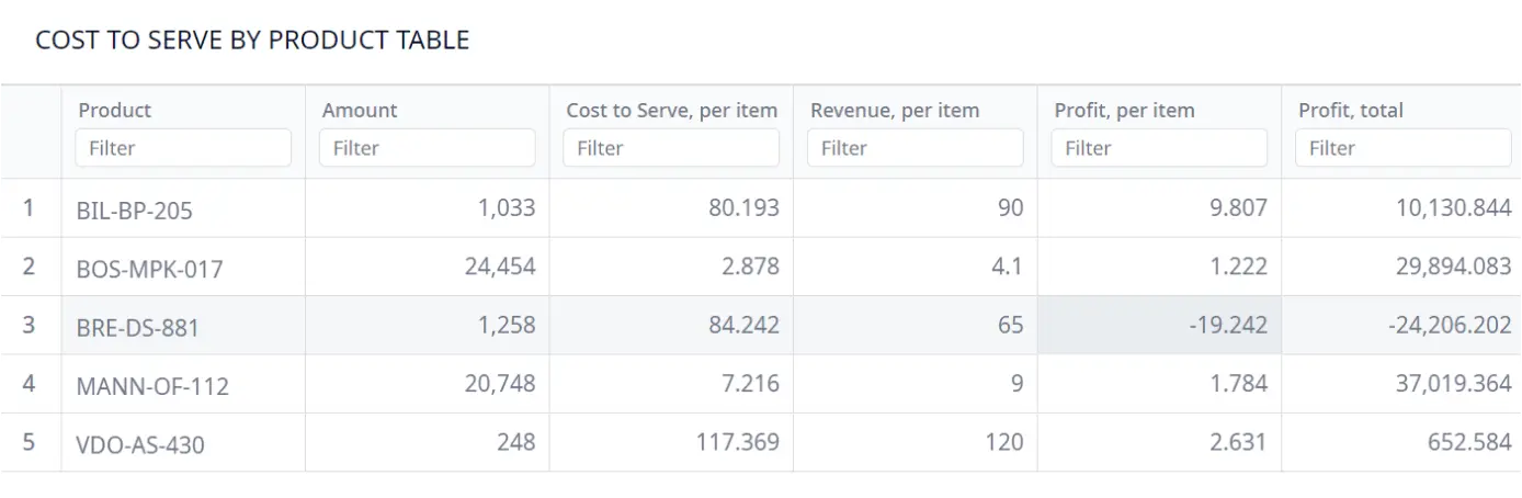
Cost to serve by product table (click to enlarge)
Another way to look at the results of cost to serve analysis is from the final customer perspective. For this, let’s use the Cost to serve by destination table that aggregates data by customer location. Sorting customers by ascending Profit, the total values show that 3 out of 24 customers are unprofitable. The total loss from serving these 3 customers is €1,552.90 (675.58 + 560.14 + 317.17).
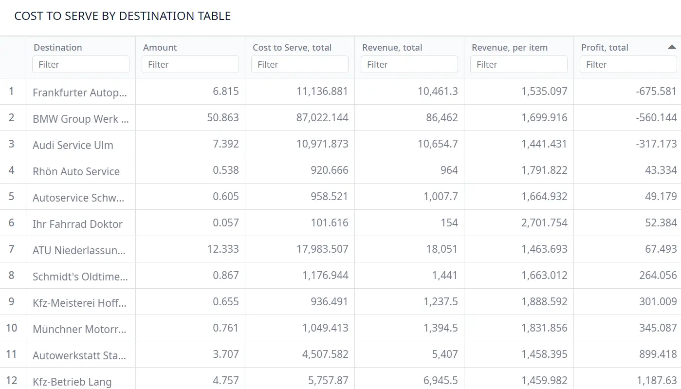
Cost to serve by destination table (click to enlarge)
However, comparing the customer-related losses (€1,552.90) with the much larger losses generated by the BRE-DS-881 product (€24,206.20) demonstrates that the company’s primary profitability issue is product-related.
Want to explore more how-to blogs and follow best practices? Discover our how-to blog post on last-mile food delivery optimization.
Cost to serve analysis is a method used to calculate the actual cost of serving customers, products, or destinations by accounting for logistics, warehousing, transportation, inventory, and service activities. Unlike traditional financial reporting, it goes beyond revenue and gross margin metrics to reveal true profitability.
Traditional profitability analysis usually focuses on high-level metrics such as revenue, gross margin, or overall profit. Cost to serve analysis goes deeper by allocating operational and logistics costs directly to customers and products. This makes it possible to identify situations where customers with high revenue may actually reduce profitability due to excessive service or distribution costs.
Supply chain design and simulation software such as anyLogistix allows companies to conduct cost to serve analysis while accounting for transportation flows, inventory, warehousing, and operational constraints. This provides more realistic insights and supports cost to serve optimization across the supply chain.
Cost to serve optimization helps organizations identify and reduce inefficiencies throughout the supply chain. By understanding the true cost of serving products and customers, companies can adjust pricing strategies, redesign networks, optimize transportation, improve service policies, and focus resources on more profitable activities.
This is how you can perform cost to serve analysis in anyLogistix and come to straightforward conclusions fast by looking at your operations from different angles. With cost to serve optimization, companies can continuously refine pricing, logistics, and customer service strategies.
Try applying the hints from the blog and explore this pre-defined case by importing it from the library of available examples in the software.
The good news? Now, no download is required to explore the power of anyLogistix. Try online, for free, in anyLogistix Sandbox.